Notes on AllStarLink DSP in chan_simpleusb.c
There are some important DSP functions in the Simple USB channel but those functions don’t have much documentation to explain how they work. This page contains my analysis.
Audio Level Statistics
Transmit and receive audio statistics are provided in the ASL Tune menus. The tune feature shows statistics on the audio levels going in and out of the USB interface, once per second. The methodology for these statistics is documented here so that alternate implementations can be fully consistent.
These calculations are performed in the chan_simpleusb audio chain very soon after a frame is captured from the USB sound card on audio receive and immediately before a frame is sent to the USB sound card on audio transmit.
The statistics are computed on a 20ms frame of 48k audio. The audio samples are in 16-bit PCM (signed) format at this point in the chain.
The frame statistics are stored in a circular buffer of length 50. The system always has one second (50 x 20ms) of statistical data available.
The 48k audio frame is down-sampled to an 8k audio frame (160 samples) by reading every 6th sample. There is no filtering applied to this down-sample operation. All statistics are computed on the 8k frames.
There are three frame-level statistics being tracked:
- Peak absolute value
- Average power
- The number of clips
The peak absolute value is straight-forward.
The frame average power is computed by summing the squares of the audio samples and dividing by 160. This calculation is performed using double-precision floating point, but the final result is converted back to q15 format.
A clip event is defined as two consecutive audio samples with an absolute value greater than 32,432. So a single audio sample of 32,767 isn’t considered a clip using this methodology.
The system displays the audio statistics every second. This requires an aggregation of the previous 50 frame statistics to form a summary for the second.
The aggregate peak power is displayed in dBFS. This is computed by finding the the maximum peak voltage across all 50 frame statistics, squaring that peak, normalizing by 230, and taking the 10×log10 of that value. A zero peak power is displayed as -96dB.
The aggregate average power is displayed in dBFS. This is computed by averaging the average powers of the 50 frame statistics, normalizing by 230, and taking the 10×log10 of that value. All steps in this calculation are performed using double-precision floating point. A zero average power is displayed as -96dB.
The maximum and minimum values of the individual frame average powers are also computed. These are used to display aggregate maximum and minimum average powers in dBFS following the same method.
The aggregate clip count is determined by summing the frame-level clip events.
The 230 factor is the square of the usual 215 factor used to normalize a 16-bit (q15) fixed point representation. The absolute audio values range from 0 to 32,767 (give or take) but we need a range from 0 to 1 to compute dBFS.
The summary display format is:
"AudioStats: Pk %5.1f Avg Pwr %3.0f Min %3.0f Max %3.0f dBFS ClipCnt %u"
prefixed by either “Rx” or “Tx” depending on the direction of the flow.
Upsampling (Interpolation) High-Pass Filter
The USB audio devices run at a 48 kHz sample rate. The IAX network audio runs at 8 kHz. Network audio needs to be upsampled by a factor of 6 as it is received. As per normal multi-rate technique, a low-pass filter needs to be applied after the 8kHz data has been expanded to 48kHz. An FIR filter is used. The comment says: “2900 Hz passband with 0.5 db ripple, 6300 Hz stopband at 60db.” The coefficients from the actual code are here:
#define	NTAPS 31
static short h[NTAPS] = { 103, 136, 148, 74, -113, -395, -694,
        -881, -801, -331, 573, 1836, 3265, 4589, 5525, 5864, 5525,
        4589, 3265, 1836, 573, -331, -801, -881, -694, -395, -113,
        74, 148, 136, 103 };
How were those coefficients determined? After some experimentation, I can match these coefficients very closely by assuming a 31-tap FIR filter with a cut-off of 4,300 Hz and a Kaiser window with a beta of 3.0. Here are the plots of the two impulse responses superimposed:
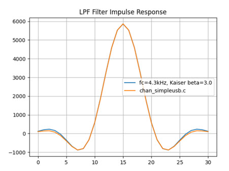
Fixed-point math is used in this filters. Input audio is 16-bit (signed) PCM and the coefficients are 16-bit signed values. After the convolution of the PCM audio and the taps is completed a final »15 operation is performed to keep the scaling right.
Downsampling (Decimation) Low-Pass Filter
It’s the opposite of above. All of the ASL processing happens at 8kHz but the USB sound hardware runs at 48kHz. So we need to decimate down the captured audio.
This process appears to use exactly the same LPF design as the upsampling filter. This filter is applied to the 48kHz input audio.
CTCSS Elimination High-Pass Filter
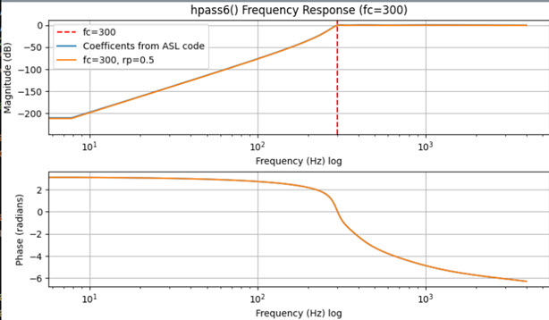
This happens in hpass6() and is selectively enabled. The goal is to strip the sub-audible CTCSS tone from the audio input. From the comment in the code this is an “IIR 6 pole High pass filter, 300 Hz corner with 0.5 db ripple.”
Taking the coefficients from the code and reformatting them a bit so that they are in the customary Direct Form I (“b/a”) used for IIR filters gives this:
b = [0.5727761454663172, -3.4366568727979034, 8.591642181994757, -11.455522909326344, 8.591642181994757, -3.4366568727979034, 0.5727761454663172 ]
a = [1.0, -4.86645111, 9.98966956, -11.06859818, 6.99051266, -2.39325566, 0.34918616 ]
- Unlike the other filter functions, this part of the code uses floating point.
- Note the “gain” variable in the code that was used to adjust the b coefficients.
- Watch out for the sign convention on the a coefficients. The coefficients shown above are the negatives of what is actually in the code to adhere to the standard b/a form.
These parameters match almost exactly with what comes out when we synthesize a 6th order Chebyshev filter using the scipy.signal.cheby1() function with fc=300 Hz and rp=0.5 dB. The frequency response curves of the filter with the coefficients from chan_simpleusb.c and the filter synthesized by SciPy are plotted below. The plots overlap perfectly:
Deemphasis Low-Pass Filter
Deemphasis is used in some systems when FM discriminator output is used directly. The feature is enabled via configuration. The code is found in deemph(). The comment in the code says “6db/octave de-emphasis” which is consistent with the standard.
The code implements a one-pole IIR low-pass filter in “Direct Form II.” The implementation uses fixed point. Reformatting the coefficients in the code into standard form we get this:
b = [ 6878, 0 ]
s = [ 1, -25889 ]
I’m not completely sure why the b1 coefficient is zero.
It’s not immediately obvious, but the code scales the output of the filter by a factor of 3. The comment is “adjust gain that we have unity @ 1KHz.”
The final output is shifted left »15 to properly normalize the values.
Here’s the plot of the frequency response:
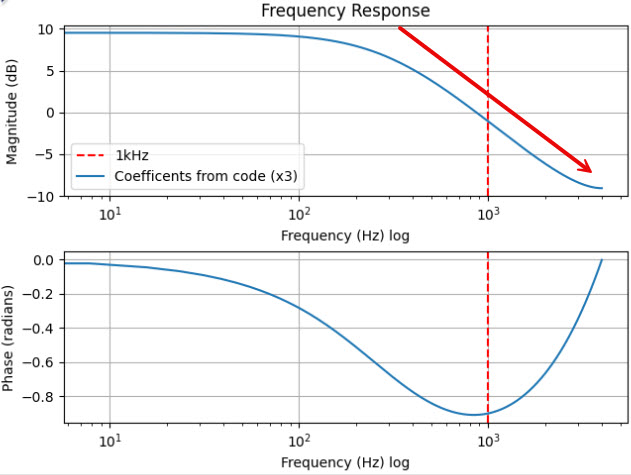
The -6dB/octave roll-off looks right and the 0dB point is right around 1kHz as documented.
Preemphasis High-Pass Filter
The purpose is the same as above, only in reverse. The implementation is different. The code is found in the preemph() function.
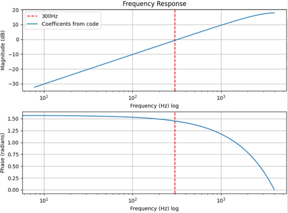
The code implements an FIR high-pass filter with two taps. Formatting into Direct Form I gives these parameters:
b = [ 17610, -17610 ]
There’s also an adjustment value of 13404 that is applied resulting in a gain of about 2.4x in the filter. This puts the 0dB point at around 300 Hz.
The implementation of this filter clips the result to between -32,767 and 32,767.
The implementation is in fixed point. The result is scaled down by »15 at the end as expected.
Here’s the plot of the frequency response:
DTMF Detection/Decoding
This is handled by the core Asterisk code (main/dsp.c) in code written by Mark Spencer himself. DTMF decoding is a complicated topic given that there are different interpretations of the “standard.” I’ve looked at the Asterisk DTMF detection code and can summarize some of the key behaviors:
- The implementation assumes 16-bit PCM audio sampled at 8kHz.
- The Goertzel algorithm is used with a block size of 102 samples.
- The row and column signals both need to exceed -8dBFS.
- Standard twist/reverse twist thresholds of 4dB/8dB are used.
- The loudest row and loudest column tones must stand out by +8dB vs the other possible tones in the same row/column.
- There is an overall S/N test applied (more research needed here)